Regression Analysis
Predicting Model for Daily Delay Count
From the previous data exploration and data analysis, we know that there exists some interesting relationship between bus delay and weather, location, and a variety of reasons. Here, we want to explore the dataset deeper to predict the number of daily delays in Manhattan as our outcome and month, weekday, daily precipitation, daily snow depth, and minimum temperature as predictors.
Our interested dependent variable is the number of delays across three school years: the number of delays in Manhattan. Based on the graph below, the daily delay across three consecutive school year have declined.
daily_df = df %>%
  filter(school_year!="2021-2022",
         boro =="Manhattan") %>%
   group_by(occur_date,school_year) %>%
   summarize(n=n()) %>%
    ggplot(aes(x=occur_date, y=n,fill=school_year))+
    geom_bar(stat='identity')+
    facet_grid(~school_year)+
      labs(
        title = "Number of Daily Delay",
        x = "Date of Delay",
        y = "Count"
      )
daily_df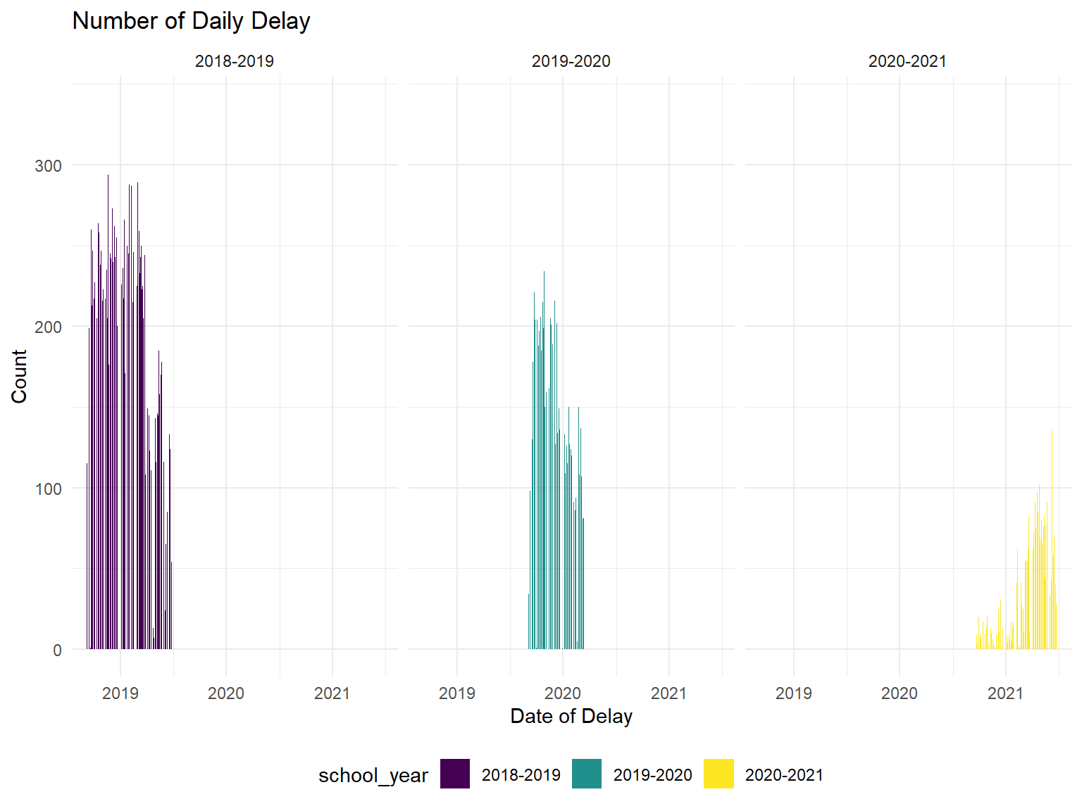
Here’s the predictors in our model:
·month: month of the incident occurred;
·day: weekday of the incident occurred;
·prcp:precipitation (tenths of mm)
·snwd: snow depth (mm)
·tmin Minimum temperature (tenths of degrees C)
Fitting Model
We propose 3 models for prediction:
1. Linear Model of daily_delay ~ month + day + snwd + tmin
2. Linear Model of daily_delay ~ month + day + snwd + tmin+ tmin*day,assuming that there are interaction
3. Linear Model of daily_delay ~ month + day + prcp
Model_1
daily_delay=df %>%
  group_by(occur_date) %>%
  mutate(daily_delay=n())

lm_1=lm(daily_delay ~ month + day  + snwd + tmin,data=daily_delay)
lm_1 %>% broom::tidy() %>% knitr::kable(digits = 2)| term | estimate | std.error | statistic | p.value |
|---|---|---|---|---|
| (Intercept) | 131.71 | 1.15 | 114.35 | 0 |
| monthDecember | 73.71 | 1.27 | 58.06 | 0 |
| monthFebruary | 71.29 | 1.29 | 55.31 | 0 |
| monthJanuary | 56.93 | 1.28 | 44.57 | 0 |
| monthJune | 30.11 | 1.54 | 19.58 | 0 |
| monthMarch | 53.46 | 1.25 | 42.80 | 0 |
| monthMay | 38.77 | 1.31 | 29.65 | 0 |
| monthNovember | 94.69 | 1.18 | 80.57 | 0 |
| monthOctober | 110.83 | 1.16 | 95.51 | 0 |
| monthSeptember | 106.81 | 1.33 | 80.12 | 0 |
| dayMonday | 14.99 | 0.76 | 19.69 | 0 |
| dayThursday | 2.90 | 0.75 | 3.89 | 0 |
| dayTuesday | 9.36 | 0.75 | 12.47 | 0 |
| dayWednesday | 4.08 | 0.74 | 5.48 | 0 |
| snwd | -0.51 | 0.01 | -44.45 | 0 |
| tmin | -3.51 | 0.06 | -61.90 | 0 |
Model_2
daily_delay=df %>%
  group_by(occur_date) %>%
  mutate(daily_delay=n())
lm_2=lm(daily_delay ~ month + day+ snwd + tmin+tmin*day,data=daily_delay)
lm_2%>% broom::tidy() %>% knitr::kable(digits = 2)| term | estimate | std.error | statistic | p.value |
|---|---|---|---|---|
| (Intercept) | 125.22 | 1.21 | 103.61 | 0 |
| monthDecember | 72.58 | 1.26 | 57.44 | 0 |
| monthFebruary | 71.68 | 1.28 | 55.87 | 0 |
| monthJanuary | 56.12 | 1.27 | 44.14 | 0 |
| monthJune | 30.30 | 1.54 | 19.73 | 0 |
| monthMarch | 52.43 | 1.24 | 42.18 | 0 |
| monthMay | 38.03 | 1.30 | 29.22 | 0 |
| monthNovember | 94.20 | 1.17 | 80.56 | 0 |
| monthOctober | 111.27 | 1.15 | 96.36 | 0 |
| monthSeptember | 106.22 | 1.33 | 79.94 | 0 |
| dayMonday | 24.35 | 1.02 | 23.87 | 0 |
| dayThursday | 6.81 | 0.95 | 7.18 | 0 |
| dayTuesday | 24.06 | 0.96 | 25.01 | 0 |
| dayWednesday | 11.61 | 0.94 | 12.34 | 0 |
| snwd | -0.51 | 0.01 | -44.77 | 0 |
| tmin | -2.45 | 0.08 | -29.42 | 0 |
| dayMonday:tmin | -1.42 | 0.10 | -14.03 | 0 |
| dayThursday:tmin | -0.58 | 0.09 | -6.33 | 0 |
| dayTuesday:tmin | -2.30 | 0.09 | -24.26 | 0 |
| dayWednesday:tmin | -1.16 | 0.09 | -12.76 | 0 |
Model_3
daily_delay=df %>%
  group_by(occur_date) %>%
  mutate(daily_delay=n())
lm_3=lm(daily_delay ~ month + day+ prcp,data=daily_delay)
lm_3%>% broom::tidy() %>% knitr::kable(digits = 2)| term | estimate | std.error | statistic | p.value |
|---|---|---|---|---|
| (Intercept) | 104.95 | 1.13 | 93.02 | 0 |
| monthDecember | 95.89 | 1.26 | 76.40 | 0 |
| monthFebruary | 85.93 | 1.27 | 67.76 | 0 |
| monthJanuary | 90.24 | 1.21 | 74.78 | 0 |
| monthJune | -8.15 | 1.47 | -5.54 | 0 |
| monthMarch | 69.26 | 1.26 | 54.98 | 0 |
| monthMay | 19.62 | 1.32 | 14.84 | 0 |
| monthNovember | 101.28 | 1.21 | 83.53 | 0 |
| monthOctober | 95.53 | 1.18 | 81.12 | 0 |
| monthSeptember | 69.04 | 1.24 | 55.53 | 0 |
| dayMonday | 13.89 | 0.79 | 17.62 | 0 |
| dayThursday | 3.72 | 0.77 | 4.81 | 0 |
| dayTuesday | 8.62 | 0.78 | 11.05 | 0 |
| dayWednesday | 5.19 | 0.78 | 6.70 | 0 |
| prcp | 0.06 | 0.00 | 19.14 | 0 |
cv_df=df %>%
  sample_n(size = 100) %>%
  group_by(occur_date) %>%
  mutate(daily_delay=n()) %>%
  modelr::crossv_mc(n = 100) %>%
  mutate_if(is.character, as.factor) %>%
  mutate(train = map(train, as.tibble),
         test = map(test, as.tibble)) %>%
  mutate(lm_1 = map(.x = train,~ lm(daily_delay ~ month + day  + snwd + tmin,data = .x)),
         lm_2 =map(.x = train,~ lm(daily_delay ~ month + day+ snwd + tmin+tmin*day,data = .x)),
         lm_3 =map(.x = train,~ lm(daily_delay ~ month + day+ prcp, data = .x)))
cv=cv_df %>%
select(starts_with("lm")) %>%
pivot_longer(
starts_with("lm"),
names_to = "model",
values_to = "data") %>%
mutate(data = map(data,broom::tidy))Cross Validation
The predictors we chose above are statistically significant.However, we notice that interaction terms are not contributing to model predictability. We would say lm_3 will be better than the other two models because its root means square error seems to be smaller. Therefore, lm_3 could be useful for predicting the total number of bus delays in Manhattan.
cv_df %>%
  mutate(
    rmse_lm1 = map2_dbl(lm_1, test, ~rmse(model = .x, data = .y)),
    rmse_lm2 = map2_dbl(lm_2, test, ~rmse(model = .x, data = .y)),
    rmse_lm3 = map2_dbl(lm_3, test, ~rmse(model = .x, data = .y))) %>%
  select(starts_with("rmse")) %>%
  pivot_longer(
    everything(),
    names_to = "model",
    values_to = "rmse",
    names_prefix = "rmse_") %>%
  mutate(model = fct_inorder(model)) %>%
  ggplot(aes(x = model, y = rmse)) + geom_violin()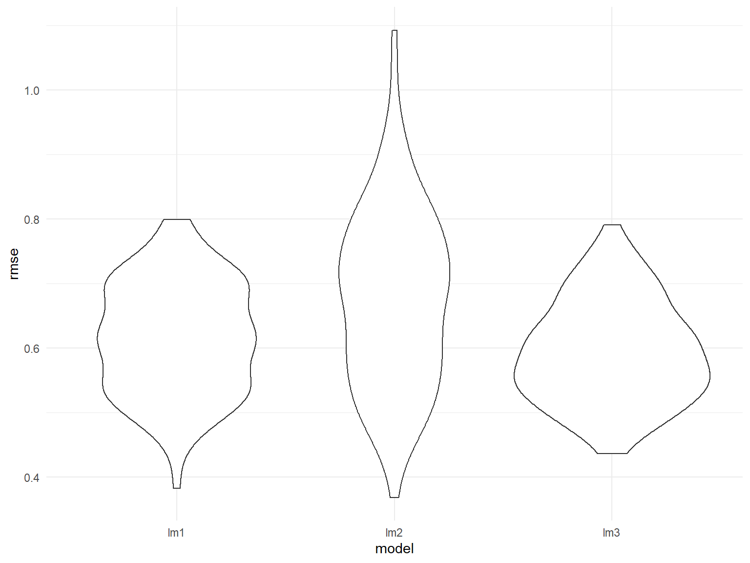
Model Conclusion
Month, rainfall, snow depth, and day are good predictors for anticipating the number of daily delays in Manhattan.